Numbers to Know
Estimation is a way to expose constraints, not a memory contest about hardware constants.
Estimation is a way to expose constraints, not a memory contest about hardware constants. Write the units beside every number and distinguish average traffic, peak traffic, and sustained overload. Use a small number of explicit assumptions to decide whether one database, a worker pool, or a provider budget is the limiting resource.
Learning goals
Units; average and peak QPS; concurrency from rate and latency; storage and retention; replication overhead; queue drain time; uncertainty.
The mechanism at a glance
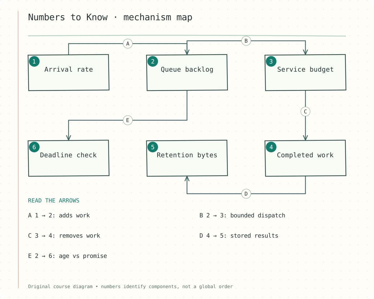
Figure — Arrival rate → Queue backlog (adds work); Queue backlog → Service budget (bounded dispatch); Service budget → Completed work (removes work); Completed work → Retention bytes (stored results); Queue backlog → Deadline check (age vs promise)
The numbered components identify responsibilities. Follow the labeled arrows rather than treating the numbers as a global execution order. The scenario later in this lesson shows one concrete sequence.
Step-by-step reasoning
1. Convert daily volume into rates
Divide requests per day by 86,400 to obtain average requests per second. Then state a plausible peak factor rather than treating the average as capacity. A regional launch or campaign can have a very different traffic shape from ordinary browsing. Separate user requests from downstream operations; one page may trigger several database reads.
2. Estimate concurrency from latency
In a stable system, average in-flight work is approximately arrival rate multiplied by average time in system. At 500 requests/s and 0.2 seconds, expect about 100 in-flight operations. This is not a universal thread count or a tail-latency guarantee. Queue waiting is part of total latency, and unstable overload invalidates a steady-state assumption.
3. Account for storage and bandwidth
Multiply records per day by bytes per record and retention days. Add indexes, replication, metadata, and working headroom separately rather than hiding them in an unexplained multiplier. Distinguish decimal GB from binary GiB when precision matters. For blobs, transfer bandwidth may dominate metadata QPS.
4. Calculate backlog and drain time
If arrivals exceed service rate, backlog grows at the difference. Once arrivals stop, drain time is backlog divided by service rate; if arrivals continue below capacity, divide by spare capacity instead. Adding workers cannot overcome a fixed provider limit. Name the admission policy when the queue age would exceed the product deadline.
Contracts and state
The following sketch makes the decision boundary concrete. Field names and capacity assumptions are illustrative; adapt them to the stated product contract.
Campaign: 1,000,000 messages
Provider limit: 500 messages/s
Best-case dispatch floor: 1,000,000 / 500 = 2,000 s
2,000 s = 33 min 20 s (before retries and overhead)

Arrivals 12,000/s; service 8,000/s
One-hour backlog growth = 4,000 * 3,600 = 14,400,000
Worked example
A million-recipient campaign must finish in ten minutes. Even with unlimited workers, a 500/s provider budget can submit only 300,000 messages in that window. The design needs a changed deadline, a higher contracted budget, or a carefully coordinated alternative provider. A larger queue merely holds the unmet promise. This is the moment where arithmetic should change the architecture or requirement.
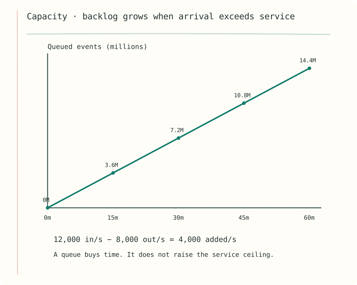
Figure — Keep arrival rate, service rate, and queue growth in distinct units.
Failure walkthrough
Averages can conceal saturation. A worker pool averaging 50% utilization may still fail if most traffic arrives in a short burst or all expensive jobs target one partition. Track queue age, per-partition load, p95/p99 latency, and error rate. Present a sensitivity range: if message size doubles, which storage or bandwidth number changes, and which capacity limit does not?
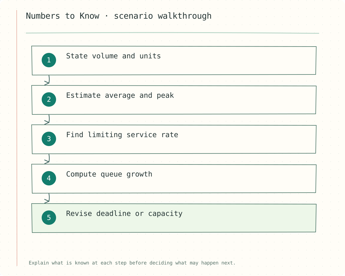
Figure — State volume and units → Estimate average and peak → Find limiting service rate → Compute queue growth → Revise deadline or capacity
Decisions and trade-offs
| Quantity | Formula | Common mistake |
|---|---|---|
| Average QPS | daily requests / 86,400 | Calling it peak capacity |
| Concurrency | rate × average latency | Mixing ms with seconds |
| Drain with arrivals | backlog / (service - arrivals) | Ignoring ongoing work |
Check your understanding
A queue contains 60,000 jobs, workers finish 500/s, and new work arrives at 300/s. How long to drain?
Show answer and explanation
Answer: 300 seconds: spare capacity is 200 jobs/s, so 60,000/200 = 300. Dividing by 500 would incorrectly assume no new work arrives. If arrivals reach or exceed 500/s, the backlog does not drain under these assumptions.
Transfer to a new scenario
Estimate a one-million-message campaign against a 500-message/s provider budget and expose the completion-time lower bound.
Why can adding workers leave campaign completion time unchanged?
Continue the connection
Study Scaling Writes and explain which guarantee from this lesson carries into that topic.
Turn arithmetic into an architectural decision
Always carry units. Ten million events/day divided by 86,400 seconds/day is about 116 events/s. A 10× peak is about 1,157/s. At 1 KB/event, raw volume is 10 GB/day using decimal units. Three replicas make 30 GB/day before indexes, logs and retention; compression changes the payload term but not every overhead equally.
Little’s Law relates average concurrent work L to throughput λ and average time W in a stable system: L = λW. At 2,000 requests/s and 200 ms average service time, expect about 400 in-flight requests. This is not a p99 sizing formula and breaks as a simple steady-state planning shortcut when backlog grows without bound.
Queues require a second calculation. If arrival is 12,000/s and service 8,000/s, backlog grows by 4,000/s. After an hour it is 14.4 million. If service later rises to 16,000/s while arrival remains 12,000/s, ideal drain time is another hour. Autoscaling must respect downstream quotas, not just queue length.
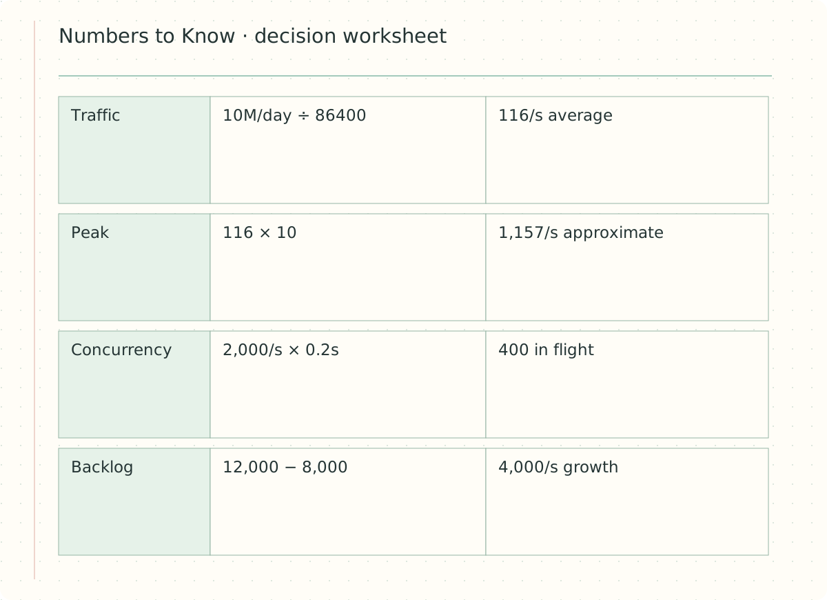
Figure — A decision worksheet for Numbers to Know: read the mechanism and its guarantee together.
Operational sketch
average_qps = daily_requests / 86400
peak_qps = average_qps * stated_peak_factor
raw_bytes = events * bytes_per_event
inflight ≈ throughput_per_second * mean_seconds
drain_seconds = backlog / (service_rate - arrival_rate)
A tempting mistake
Do not multiply every pessimistic factor without explaining the scenario, and do not confuse bits/s with bytes/s. A fleet average can hide one hot tenant or one overloaded shard.
Transfer exercise
A provider allows 500 requests/s. Workers take 0.2 seconds per call. Is 10,000 concurrency useful?
Show answer and explanation
Answer: About 100 in-flight calls supports the ideal quota rate at that mean latency. Extra headroom may absorb variation, but 10,000 concurrent calls cannot lawfully raise the quota and can magnify retries.